Excel formula for matching data
I've made a table with names in the first row.Critiques : 128
Excel MATCH function with formula examples
Applying the FILTER Function to Lookup Multiple Values in Excel.=VLOOKUP (E2,A2:C5,3,FALSE) The formula uses the value Mary in cell E2 and finds Mary in the left-most column (column A).
COUNTIF function
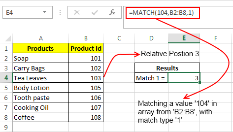
In financial analysis, we can use the MATCH function along with other functions to look up and return the sum of values in a column. Compare Sheets with the Match Function. Decide in which list you want to highlight matching or non-matching records. In the example shown, the formula in G7 is: =XLOOKUP(H4,data[Name],data,,,-1) Where data is an Excel Table in the range B5:B16. Try using the CLEAN function or the TRIM function. Both are considered the same. Step 1: Select all of the cells you want the Conditional Formatting to apply to. It is commonly used with the INDEX function. MATCH supports approximate and exact matching, and wildcards (* ?) for partial matches.= MATCH (B7, A2:A5, 0) Pro Tip! The MATCH function has three different match types 3️⃣. VLOOKUP formula to compare 2 columns. Step 4:
How to copy row data matching specific column criteria
For instance, you might look up the value 10 in the cell range B2 . Criteria1, criteria2, .
How to Compare Two Columns in Excel (for matches
Quick Conditional Formatting to compare two columns of data. You may use the FILTER Function to filter a set of data depending on the criteria you give to seek numerous values. 1 Using Conditional Formatting.
MATCH Function
Excel VLOOKUP with SUM or SUMIF function
If you want to highlight records in only one list, you'll probably want to highlight the records unique to that list; that is, records that don't match records in the other list.
Make sure your data doesn't contain erroneous characters. In the example shown, the formula in J8 is: =INDEX(C6:G10,MATCH(J6,B6:B10,1),MATCH(J7,C5:G5,1)) Note: this formula is set to approximate match, so row values and column values must be sorted. Col_index_num: This is the column number in the table_array from which the matching data should be . If you want to match . Match data in Excel using the MATCH function.VLOOKUP examples.
The general argument of the function is, =EXACT(text1,text2) Now insert the values into the function and the final form .
(Exact/Partial Match)
=CONCAT(C2,B2) OpenAI.Comparison can be done in many different ways - which method to use depends on exactly what you want from it. The above formula will give you a TRUE if both the values are the same and FALSE in case they . If you have two datasets and you want to compare items in one list to the other and fetch the matching data point, you need to use the lookup formulas.
How to compare two columns in Excel using VLOOKUP
For more information, see VLOOKUP function. INDEX and MATCH examples. 2 Using VLOOKUP. For example: =IF(B2=C2, Same score, ) To check if the two cells contain same text including the letter case, make your IF formula case-sensitive with the help of the EXACT function. The formula then matches the value in the . Basic Syntax: =VLOOKUP(lookup_value, table_array, col_index_num, [range_lookup]) Application: Go to the cell in Worksheet 2 where you want to display the matched data. This is because INDEX and MATCH are incredibly flexible – you can do . Step 2: Use the “Merge” command to select the columns you want to match. TRIM is used to remove extra spaces from the start, middle, and end. sometimes, I only have the family's last name). I want to copy these rows to another worksheet.That is-“Arizona” ROW(INDEX(State,1,1)) Then the ROW function will find its original row number- {5} ROW(State)-ROW(INDEX(State,1,1))+1 As the upcoming INDEX function works for row . I need help to write an Excel formula that will do the following: If a date in the data matches a date in the date range, I need a formula that will place the option S or BS at the correct place under the correct name. The steps to compare and match data in Excel using the VLOOKUP function and the Subtraction operator, ‘–‘, are as follows:. It's a GREAT formula; I'm simply hoping to use more data to get stronger matches.
How to Find Matching Values in Two Worksheets in Excel
Often, MATCH is . My list of 10 names: Sam . In the example shown, the formula in H7 is: =VLOOKUP (value&*,data,2,FALSE) where value (H4) and data . Step 4: Drag the formula down or across.Method #1 – Match Data Using VLOOKUP Function. Copy the data lists onto a single worksheet. Download this VLOOKUP calculations sample LOOKUP AND SUM - look up in array and sum matching values.When looking up some information in Excel, it's a rare case when all the data is on the same sheet.I'll copy only the row data matching anyone in that list of 10 names. The syntax for the MATCH function is . search across column 2 for any matching WORD (not the full name! this would not be .
Excel INDEX MATCH with multiple criteria
The good news is that Microsoft Excel provides more than one way to do this, and the bad news is that all the ways are a bit more complicated than a .Steps: In cell F5, apply the EXACT function.Use the VLOOKUP Function.Below is a simple formula to compare two columns (side by side): =A2=B2.If we add the above formulas to the 'Summary Sales' table from the previous example, the result will look similar to this:. See the syntax, arguments, examples, and tips .; Enter the following VLOOKUP() formula in the chosen cell. 1 (or omitted) – Search for the largest value less than or equal to the lookup .To find the closest match to a target value in a data column, use INDEX, MATCH, ABS and MIN in Excel.
How to Use the MATCH Function in Excel (Formula)
Prepare your two worksheets in the same workbook. The function will then search for the lookup value in the specified table array and return the corresponding value from the specified column. Clearing the Conditional Formatting. To do this, I .The most popular way to do a two-way lookup in Excel is by using INDEX MATCH MATCH. From formulas and Conditional Formatting to Power Query.To get the last match in a set of data you can use the XLOOKUP function. Enter the VLOOKUP formula, where: lookup_value is the value in Worksheet 2 you want to match against Worksheet 1. Table_array: This is the range of cells that contains the data you want to retrieve information from. In the example shown, the formulas in K11 and K12 are, respectively: = INDEX ( data, .; After that, we used the ISNUMBER function to check if the result of the SEARCH function is a number.Very often there is a requirement in Excel to compare two lists, or two data sets to find missing or matching items.
Excel Formula for Matching
By using formulas like VLOOKUP, you can easily compare two sheets in Excel and identify any matches, saving you time and effort.How to Find Matching Values in Two Columns in Excel.Given a range of dates and data including names, two options S/BS, and dates.Simply type the following formula to return a TRUE (if they match) or FALSE (if they don’t). After writing the VLOOKUP formula, enter it into the cell where you want the matched data to appear.
MATCH function
VLOOKUP function
Beginners Guide: How To Compare Two Excel Sheets For Matching Data
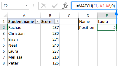
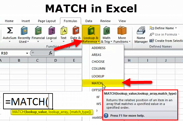
More often, you will have to search across multiple sheets or even different workbooks.Compare Two Columns and Pull the Matching Data. Type this string in the second argument, and you will get this simple .To create a formula that checks if two cells match, compare the cells by using the equals sign (=) in the logical test of IF.Step 3: Enter the VLOOKUP formula in Excel. Another way to do a two-dimensional lookup in Excel is by using a combination of VLOOKUP and MATCH functions: VLOOKUP ( vlookup_value, table_array, MATCH ( hlookup_value, lookup_row_range, 0), FALSE) For our sample table, the formula takes the following shape: =VLOOKUP(H1, .Learn how to use the MATCH function to find the relative position of a value in a range of cells, and return the value or the position.The MATCH function in Excel searches for a value in the array, or range of cells, that you specify.
3 Easy Ways to Find Matching Values in Two Columns in Excel
Enter the Following Index Match Formula method to compare the two . It is commonly used to identify duplicate values in cells, and for some reason, extra space makes it unique.

The VLOOKUP formula consists of four main components: Lookup_value: This is the value you want to search for in the first column of the table. =VLOOKUP(lookup_value_dataset2, table_array_dataset1, col_index_num, .To lookup in value in a table using both rows and columns, you can build a formula that does a two-way lookup with INDEX and MATCH.{=INDEX ( return_range, MATCH (1, ( criteria1 = range1) * ( criteria2 = range2) * (. The Dynamic Arrays Function contains this function. When counting text values, make sure the data doesn't contain leading spaces, trailing spaces, inconsistent use of straight and curly quotation marks, or nonprinting characters. Select a column where you want to put the matching data.; Then, we used the OR function to check if any of .
Excel VLOOKUP function
In Excel 365, the new FILTER function provides a more powerful way to filter on partial matches. Microsoft calls this a dynamic array and spilled array.Users can use the VLOOKUP (), INDEX + MATCH function and use these functions based on uniquely-created lookup values to match data in one or more worksheets. Dealing with Non-Matches.In its simplest form, the VLOOKUP function says: =VLOOKUP (What you want to look up, where you want to look for it, the column number in the range containing the value to return, return an Approximate or Exact . 3 Using a TRUE/FALSE .Learn how to use the IF function in Excel to check if two or more cells are equal, return custom text or values, or return another . When comparing two Excel sheets, it's inevitable that you'll come across non-matching data. If the contents of both cells match exactly (irrespective of case), the formula returns a TRUE., inner join, left join, right join). The array formula below is for earlier Excel versions, it searches for values that meet a range criterion (cell D14 and D15), the formula lets you change the column to .VLOOKUP and MATCH formula for 2-way lookup.; Similarly, we searched for Veg in Cell B5 using these two functions.

Click on “Data” and “Get Data” tab followed by selecting the data source from which you want to match the two columns. Choose a cell to apply the VLOOKUP().I need a formula that will: take the name (or separate words) from column 1.Solution: Step 1: Select the cell where you want to display the product “Deodorant” position.The formula will automatically convert a numeric value from age to string and combine it. The most recent formula, courtesy of a great person in this community a few years ago, is below. The result is an array of data that dynamically flows into a range of cells, starting with the cell where .The Excel VLOOKUP function is used to retrieve information from a table using a lookup value. “24”+“M” = “24M”. In this article we are going to look at a number ways to compare two lists in Excel . Example: Pull the Matching Data (Exact) For example, in the below list, I want to fetch the market valuation value for column 2.It is a regular formula, however, it returns an array of values and extends automatically to cells below and to the right. 0 – Search for the exact match of the lookup_value.), 0))} Where: Return_range is the range from which to return a value. The lookup values must appear in the first column of the table, and the information to retrieve is specified by column . In this case, let’s assume it is cell B12.
How to use INDEX and MATCH
Excel MATCH function
Download Article.How Does the Formula Work? In the beginning, we used the SEARCH function to find cell range Bars in Cell B5.


.jpg)