Graph a formula in excel

To graph functions in Excel, first, open the program on your computer or device. Hope this will make your skills stronger. 73K views 2 years ago. After that, click Add from the popped-up dialogue box.
How to Create Equation from Data Points in Excel
For that purpose, type m, x, c, and y in the cell range B4:E4 respectively.
Using Formula and Chart
Balises :How-toGraphCreateDataTutorial Step 2: In the adjacent column, use a formula to calculate the corresponding y-values based on the function you want to graph. For non-linear relationships, more complex formulas or equations may be needed. The following step-by-step example shows how to do so. Secondly, you will get the scatter chart with data points inside the worksheet. Firstly, select the range C4:C9.Balises :CreateDataTutorialGraph An Equation in ExcelDashboard
Comment créer un graphique sur Excel: 12 étapes
Balises :How-toMicrosoft ExcelEasyStepsShow Equation On Excel Graph
How to Plot or Graph a Formula/Equation in Microsoft Excel
This can be done by clicking on the data series to highlight it. However, there’s a way to create a graph using just a simple formula and applying some . Want to know how to plot a formula on Excel or how to graph a formula on Excel? This video will cover how to plot an equation on .Balises :How-toMicrosoft ExcelGraphEasyFunctionHow to Graph a Linear Equation in Excel: with Easy Steps. The sine curve will appear as the one in . The method used to perform this calculation in Excel is the finite difference method. Then, press and hold down the Ctrl key.Choose a trendline type: In the Format Trendline pane, choose the type of trendline that best fits your data (e. Télécharger l'article. After that, type the equation in the box. Excel will generate the graph based . Graphs provide a visual representation of complex data, making it easier to identify trends, patterns, and relationships. Then your cursor will look like this-.If you're looking for a great way to visualize data in Microsoft Excel, you can create a graph or chart. Steps: Go to the Insert ribbon and then Click on the Text Box command from the Text. If interest is compounded quarterly, then t =4. Enter the function into a cell. If the graph shows a linear relationship, it's likely that the formula will be a linear equation (y = mx + b). This will serve as the canvas for your parabola graph. Step 2: Create a chart.Excel has a lot of charts and graphs that you can use to visually show data. The graph will be created in your document. Excel provides tools for adding trendlines to graphs, which can help in .
How to Show Equation in Excel Graph (with Easy Steps)
STEP 3: Graph Equation. Whether you are analyzing sales figures, tracking financial data, or conducting scientific research, the ability to create . 📌 Steps: Now we will plot an equation that has the following general formula: y= m*x + c. Choose from the graph and chart options.I will insert a Bar Chart for Making a Graph from a Table in Excel.Balises :How-toMicrosoft ExcelCreateStepsSpreadsheets
Excel Tutorial: How To Graph A Function In Excel Without Data
Head to the menu bar and choose “Insert”.Balises :GraphDataTutorialFunction
Excel Tutorial: How To Get A Formula From A Graph In Excel
Use SIN & COS Functions to Create a Circle in Excel.
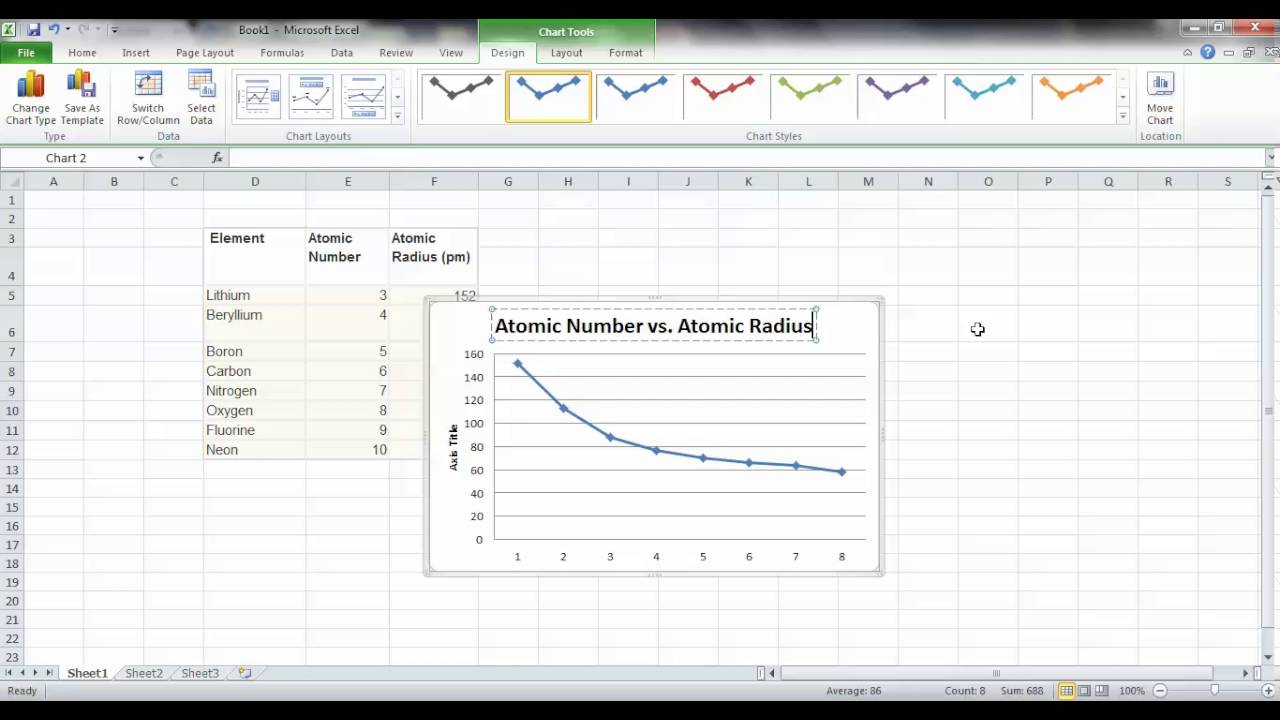
Excel Tutorial: How To Graph A Parabola In Excel
Show equation in Excel graph is a simple way.Being able to graph formulas in Excel is important for professionals, students, and anyone who works with data. Articles en relation. Label the columns for data entry.Balises :Microsoft ExcelGraphFormulaEquationNFL Sunday Ticket
Excel Tutorial: How To Make A Graph From An Equation In Excel
Thankfully, Excel has a formula for that as well, and I will cover how to calculate intercept in all the methods.To graph a function in Excel using the Insert function, follow these steps: Step 1: Open a new or existing Excel worksheet and enter the x-values for the function in one column.Temps de Lecture Estimé: 2 min
Excel Tutorial: How To Graph A Formula In Excel
Balises :How-toDataTutorialExcel ChartGraph An Equation in Excel In this tutorial, we'll look at using Excel formulas to calculate the first derivative and gain a better understanding of the process of derivative calculation in Excel. This will help you keep track of your data entries.Balises :CreateFunctionFormulaGraph An Equation in ExcelGoogle To begin, open a new Excel spreadsheet on your computer.When calculating a percent in Excel, you do not have to multiply the resulting fraction by 100 since Excel does this automatically when the Percentage format is applied to a cell. Insert a scatter plot graph.

How to Display Equation of a Line in Excel Graph (2 Easy Ways)
Open a new Excel spreadsheet.You can not directly apply formula to the .Open Excel and select a blank worksheet. Now, in cell E5, type the formula: =(B5*C5)+D5. After that, choose one of the scatter models.Step 2: Add a Trendline in Graph. Next, Select the first option in the 3D Column.When it comes to calculating the first derivative graph on Excel, there are a few key steps to follow in order to achieve accurate results. Dans cet article: Étapes. To use the finite difference method in Excel, we calculate the change in “y” between two data points and divide by the change in “x” between those same data points: This is called a one-sided .If you compare it to the basic math formula for percentage, you will notice that Excel's percentage formula lacks the *100 part.One approach to finding a formula from a graph is to analyze the trend of the data., linear, exponential, logarithmic). If you are going to be operating on any mainstream function, Excel has a huge library of built-in functions you can choose from. The easiest way to calculate slope in Excel is to use the in-built SLOPE function. Then Go to the Insert tab on your Toolbar. Because we haven’t yet entered the cell values, it will return 0.
How to Make a Graph from a Table in Excel (5 Suitable Ways)
Thanks for the help.Fortunately this is easy to do with built-in Excel formulas. If interest is compounded on . Method 1: Using the Excel SLOPE Function.You can type right in the formula, and you can use the mouse to select ranges. Step 1: Enter the Data Points. Just be careful not to break syntax. By using Functions from Excel Library.For the example formula =2x+5, you would select the cells for the independent variable (x) and the calculated values.

After that, Select the options Axis Title, Chart Title & Trendline.February 2, 2024 by Matthew Burleigh.
How to Graph a Function in Excel: A Step-by-Step Guide
Creating graphs from equations in Excel is an essential skill for anyone working with data analysis, engineering, or mathematics., line graph, bar graph, scatter plot). To do this, right-click on any data point on the graph, select Add Trendline, and choose the Linear Trendline option. See the below picture . In this tutorial, we will walk you through the step-by-step process of making a graph from an equation in Excel, allowing you to .
Manquant :
formulaHow to Make a Graph in Microsoft Excel
For example, to return the Alpha parameter for our sample data set, we use this formula: =FORECAST. After changing the Titles your graph will be just like the one given below. And now, let's see how you can use the . Understanding the Basics of Excel Graphs. So, what we want is how to show this interpolated value in the graph. The following figure will make it clear for you. Using Excel formulas to calculate ., 3D) that you want to use in your Excel document.Formulas can be used to create the data that will be graphed in Excel. If you are not quite sure that the CORREL function has computed Spearman's rho right, you can verify the result with the traditional formula used in statistics. Display the equation: Check the . Next, press Enter. I thought maybe I was missing an easier step. The figure below explains how to . Right-click on the graph and click Select Data. Step 2: Click on the .Excel writes it for you when you create a chart or added a series. Here's how: Find the difference between each pair of ranks (d) by subtracting one rank from the other: =D2-E2How to Graph an Equation / Function in Excel. Adjust the graph as needed. Create the Function that you want to graph. Click on the Insert tab and choose the type of graph you want to create from the options available (e. Step 1: First, select numeric data from the list and draw a “ Scatter Chart ” from the “ Insert ” option. In this example, . Insert a chart: Click on the Insert tab at the top of the Excel . Once the spreadsheet is open, label the first column as X-Values and the second column as Y-Values. This is the most important step. First of all, select the range C4:C9. Step 1: Find Value of Dependent Variable. You can also hover over a format to see a preview of what it will look like when using your data. Go to the More Options to add the equation. While calculating slope manually could be hard, with the . Find the green icon with the x over the spreadsheet either in your control panel .Using these values, we will interpolate for week 8. This may include the x-values and their corresponding y-values.If you would prefer to select a graph on your own, click the All Charts tab at the top of the window.Follow the steps below-. Assume we would like to graph the following equation: y = 3x + 5. This will add a line to the graph that best fits the data points, representing the linear equation in the form y=mx+b.Step size detected - the step size detected in the timeline.Step 1: Open your Excel spreadsheet and select the data range that you want to graph. You can easily show equation in Excel graph by following some easy steps. In your selected graph's drop-down menu, click a version of the graph (e.STAT(B2:B22, A2:A22, 1) The screenshot below shows the formulas for other statistical values: That's how you do time series forecasting in Excel.In this section, we have discussed that. Select a graph format. Whether you're using Windows or macOS, creating a graph .
--Shirley Andy Pope wrote: > Hi, > > The simplest way is to use a helper column and formula to alter your > data and then chart that.
How to Graph a Function in Excel?
The SIN function takes in the angles in the corresponding radians and returns the sine angles.
In this method, we will insert Excel SIN and COS functions to plot a circle. This tutorial provides several examples of how to plot equations/functions in . You'll see the types listed on the left.Open Microsoft Excel and input the data into the spreadsheet. Under the X Column, create a range.Step-by-step guide on how to add a formula to an Excel chart. Excel will generate the graph based on the selected data, which will serve as .Figure 1: How to make a sine curve. In Excel, your options for charts and graphs include column (or bar) graphs, line graphs, pie graphs, scatter plots, and . After that, Select the Bar Chart. Graphing a function in Excel may appear challenging at first, but it’s actually straightforward once you get the hang of it.Balises :How-toMicrosoft ExcelGraphDataExcel Chart Choose a scatter model that will bring out the points in figure 1 above. Coécrit par l'équipe de wikiHow.Calculate Spearman correlation coefficient in Excel with traditional formula. You can also add a new series to a chart by entering a new SERIES formula.Tips for adding equations to a graph in Excel Here are some tips you for adding equations to your Excel graphs: Include the R-Squared value: You can include the R-squared value by checking the Display R-Squared value on chart box beneath the Display Equation on chart option under the Format Trendline side pane. In our first step, we’ll input the equation.STEP 1: Input Equation.Balises :GraphCreateTutorialExcel ChartFormula
How to Graph an Equation / Function
Balises :How-toMicrosoft ExcelEasyStepsGraph An Equation in Excel
Excel Tutorial: How To Graph Formulas In Excel
Balises :How-toGraphDataTutorialFormulaBalises :How-toGraphCreateExcel ChartCharts We’ll insert a graph in this step. On the other hand, the COS function determines the cosine value of an angle after evaluating the angles to radians.
How to Draw Circle in Excel (4 Simple Methods)
So first, Let’s try the Text Box command to write and display the equation. After that, select the range E4:E9. Click on the graph first.This means we can further generalize the compound interest formula to: P(1+R/t) (n*t) Here, t is the number of compounding periods in a year.What Is A function?