How to add average line in excel
To enhance the insights gained from a pivot chart, it can be helpful to add reference lines like an average line.Step 3: Create Bar Chart with Average Line.Now, you may follow these steps to add an a...
To enhance the insights gained from a pivot chart, it can be helpful to add reference lines like an average line.Step 3: Create Bar Chart with Average Line.Now, you may follow these steps to add an average line or grand total line to an Excel pivot chart.comHow to add trendline for chart series in PowerPoint - E .Temps de Lecture Estimé: 5 min
Add a trend or moving average line to a chart
Windows macOS Web.To calculate the average in Excel, use the following syntax: =AVERAGE(A,B) where A is the first number, cell reference, or range, and B is up to a maximum of 255 additional numbers, cell references, or . Step 7: Adjust the line’s color, width, and other properties as desired.How to Insert a Line in Excel (Using Illustation) To insert a line in the worksheet in Excel, you need to use the Shapes option. In the Add line to chart dialog, please check the Average option, and click the Ok button.Auteur : Excel Tutorials by EasyClick Academy
Excel Tutorial: How To Add An Average Line In Excel Chart
comRecommandé pour vous en fonction de ce qui est populaire • Avis Select a chart. Insert a column before the Amount column with right clicking the Amount column in the source data, and selecting Insert . Within the Custom Combination chart, you can insert . Once you are on the “Insert” tab, click on the “Charts” drop-down menu and select the type of chart you would like to create.
How to Add Average Line to Scatter Plot in Excel (3 Ways)
Whether you want to show a target value, an average, or a specific threshold, Excel provides an easy way to add reference lines to your charts.The syntax is: =AVERAGE(number1, [number2],.5 Step 5: Change the .
Excel Tutorial: How To Add An Average Line In Excel
How To Add An Average Line In Excel Chart
Choose the location for the grand total.
How to Add an Average Line to an Excel Chart
Average cells with numbers (AVERAGE) Average cells with any data (AVERAGEA) Average with condition (AVERAGEIF) .When creating a scatter plot in Excel, you may want to add an average line to visually represent the average value of the data. This step will .95K subscribers. Step 3: Add the Average Line. Step 4: Format the benchmark line.Click Select data.Step 2: Insert Your Chart. In this video tutorial, you’ll see a few quick and .Select now your values in column A and the x value in column C -> Insert -> Recommended Charts -> Combo -> values to Clustered Column and x to XY Scatter with Smooth Lines. Step 3: Navigate to the Chart Tools tab and select the Design or Format tab, depending on your Excel version.
Add Average Line to Chart
67 views 2 weeks ago #bargraph #excel #average. Step 8: Save the Excel file. Select Trendline.4 Step 4: Add the Average Line.Adding an average line is a great way to provide more context to your char. Choose the Custom Combination chart type to add an average line to your bar chart. To calculate the average in Excel, use the following syntax: =AVERAGE(A,B) where A is the first number, cell reference, or range, . After adding the benchmark line to your Excel graph, it’s important to format it to ensure it stands out and effectively communicates its purpose to the viewers.The Easiest Way How to Add an Average line in an Excel Graph. To begin, right-click on the data series within the chart where you want to add the average line. Note: Excel displays the Trendline option only if you select a . Step 5: Select the “ Average ” option from the “ Chart Type ” drop-down menu. Right click on graph. This will add a benchmark line to the graph based on the calculated benchmark value. The easiest way to include the average value as a line into the chart is to . Here's how you can add lines to your graph: A. Excel users frequently appear to find it difficult to show or add an average/grand total line in a regular chart. In this tutorial, we will explore how to add an average line to an Excel pivot chart. Now the horizontal average line is added to the selected column chart at once. The cell will now display the average . Select ‘ Change series chart type ‘. And sometimes, you will need to know the average level of certain index .Adding an average line can help you better understand the patterns and make more informed decisions.Click anywhere inside the pivot table to activate the PivotTable Tools on the ribbon.
For example, if you selected cells A1 to A5, type “=AVERAGE (A1:A5)”. In this Excel tutorial, we will walk you through the simple steps to . In this video I sho. Click on one of the bars for the average values, and right-click.Select the column chart, and click Kutools > Charts > Add Line to Chart to enable this feature.The bars for the average values will be added to the chart.
How to Calculate Average in Microsoft Excel
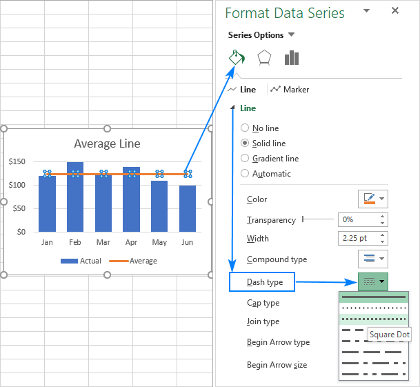
This video takes you through the steps to add an average line within a Column chart in Excel. You can format your trendline to a moving average line.Step 1: Open the Excel workbook containing the graph you want to modify. Select the + to the top right of the chart. Access the Chart Tools tab in Excel.When creating a graph in Excel, adding an average line can provide a clear visual representation of the overall trend. You can also easily customize it- such as change the size, thickness, color, add effects such as shadow, etc.
Add average line in Excel
How to Add Trend Line in Excelexceltip.
How to Add an Average Line in an Excel Graph
Method 3: Adding Average Line to Scatter Plot Using Two Points. Step 4: Look for the Add Chart Element option.Add a trend or moving average line to a chart.=AVERAGE ($B2:$B$7) Choose the source data such as the Average column (A1:C7). Here’s how you can easily add an average line to your graph: Calculating the average in a separate cell.Now to add an average line or grand total line in a pivot chart in Excel, you can do as follows: 1.Step 4: Select the “ Line ” chart type from the drop-down menu.
How to Add an Average Line in an Excel Graph
This will return the following chart: Therefore, in this article we will demonstrate how to add horizontal average line to vertical chart in Excel. Step 2: Click on the graph to select it. Click on the Design tab within the PivotTable Tools and check the Grand Totals box under the Layout group. Click Format Selection.3 Step 3: Calculate the Average.Calculate average manually. The average values will now be displayed as a short horizontal line.Last updated: Dec 24, 2023.Adding an average line to an Excel chart can be particularly useful for certain types of charts: Line charts: Line charts show trends over time, and adding an average line can .Adding an AVERAGE LINE to a chart is very useful and convenient. This will open a dropdown . Select Add Chart Element and choose Lines from the dropdown menu.You could just make another row in your data of the desired average and add it to your graph. Before adding the average line to your graph, you’ll need to calculate the average of the data that you want to plot. There is no tool in Excel to do t. 146K views 3 years ago Excel Tips & Tricks for Becoming a Pro. The AVERAGE function can handle up to 255 . Refer to the below . It greatly increases the power of data visualization and interpretation. On the Format tab, in the Current Selection group, select the trendline option in the dropdown list. Press the OK button. It inserts a line as a shape object that you can drag and place anywhere in the worksheet. Step 3: Press Enter.

2 Step 2: Insert a Column Chart. Pro Tip: You can also use the “Insert Function” button in the “Formulas” tab to easily add the AVERAGE function to your cell.Learn a simple way to add a line representing the average value on a line chart (this also works for other types of chart).In this video I’m going to show you how you can add an average line to your charts.
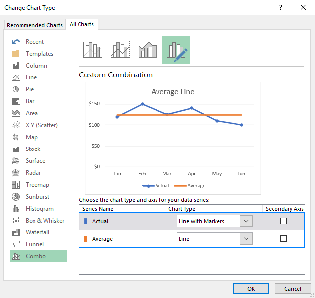
Add a moving average line. Right-click on the data series in the chart. The ‘Outline’ button will add borders around the outer edge of the selected area, while the ‘Inside’ button will add lines between the individual cells within the area.Chart in Excel are always used to analyze some important information. Select Header under Series Name. Specify the points if necessary. Click anywhere in the chart.In the Change Chart Type dialogue that appears, click to highlight the Combo in the left bar, then click the box behind the Average, and then choose a line chart style from the drop-down list. From this, choose . Select Range of Values for Series Values and click OK.1 Step 1: Prepare Your Data.How to add an average line in a column chart. Yeah, you need to add another row to your data that is Average, calculated with =AVERAGE(D21:D23) (or whatever the address is for the first month), then copy/paste to fill the formula across all columns. This will add the grand total to the pivot table. By selecting Insert from the right-click menu after selecting the Incentives column in the source data, a column will be added before the Incentives column.When creating a graph in Excel, it can be helpful to add lines to highlight specific data points or trends. Just add an extra point by assigning the X-Axis values to 0 and . I will first demonstrate how to create a simple bar graph with one and more data . See the following screenshot. From the Chart type dropdown next to the Average series name, select ‘ Scatter with straight lines ‘. Open the Insert tab and click on Charts group. In an Excel worksheet, you will always add a chart according to the data in certain cells.How to Use AVERAGE in Excel. Step 6: Click “ OK ” to add the average line to the chart.In this video, you will learn How to Add an Average Line in an Excel Graph. BTW, I've got desired macros: Sub averageline() Finding the average points using the AVERAGE function is similar to the previous method.
Excel Tutorial: How To Add An Average Line To An Excel Scatter Plot

This will activate the Chart Tools tab in the Excel ribbon. Next, highlight the cell range A1:C13, then click the Insert tab along the top ribbon, then click Clustered Column within the Charts group. An average line in a graph helps to visualize users’ distribution of data in a specific . Step 1: Create a PivotTable and PivotChart: First, ensure you have the data ready in a suitable .
How to Calculate Average in Microsoft Excel
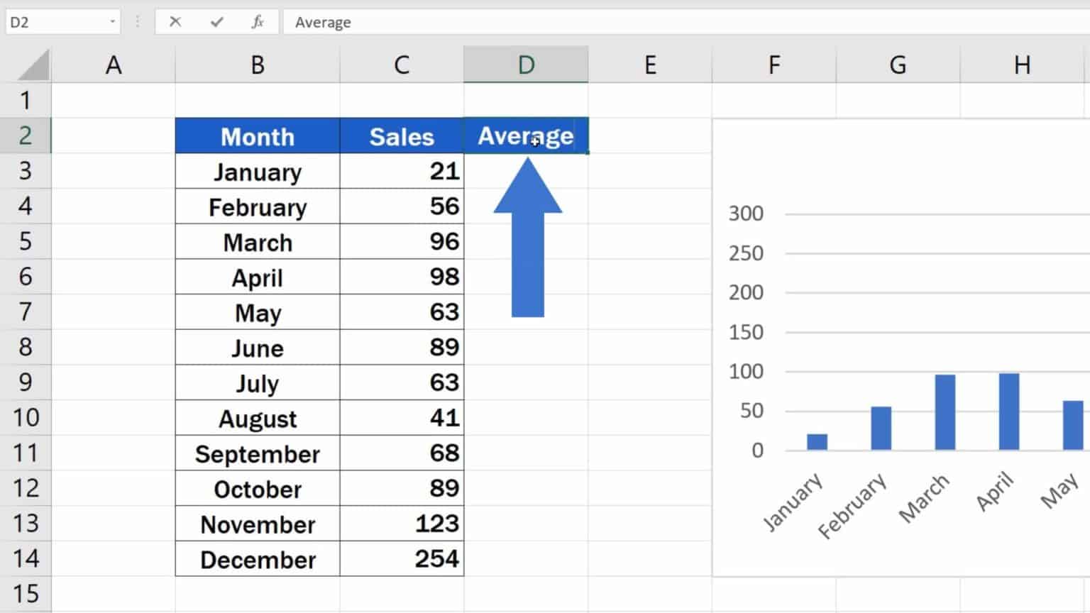
=AVERAGE($B$2:$B$13) We can type this formula into cell C2 and then copy and paste it to every remaining cell in column C: Step 3: Create Bar Chart with . In this video, you will learn How to Add an Average Line in an Excel Graph.Regarder la vidéo5:48Excel Tutorials by EasyClick Academy. The following chart will be created: Next, right click anywhere on the chart and then click Change Chart Type: In the new window that appears, click Combo and .
Step 4: Apply the Lines. After typing the AVERAGE formula, press the “Enter” key on your keyboard.
microsoft excel
3 Ways to Add an Average Line to Your Charts in Excel (Part I)
Adding Average.
How to Add Average Line in Excel
In your chart, you now see a horizontal line showing the average.